APRIL 21, 2025
EXCEL
Finding duplicates in Microsoft Excel is a crucial part of data management and data analysis.
Whether you’re cleaning up an Excel dataset, identifying duplicate records, or ensuring data integrity, knowing how to highlight duplicate values efficiently can save you a lot of time.
Excel provides various ways to identify duplicate data, including built-in features like Conditional Formatting, the Remove Duplicates tool, and Excel formulas like the VLOOKUP formula and COUNTIF formula.
In this blog post, we’ll walk through the simplest ways to find duplicate values in two different columns using effective methods.
These methods work across different versions of Excel and can be applied to large datasets.
So, let’s have a look.
You may also want to see: How to Have Multiple Lines of Text in One Excel Cell.
One of the easiest ways to highlight duplicate rows or cells is by using Conditional Formatting.
This built-in feature helps identify duplicate cells in a column visually.
Here are the steps:
Select the range of data in Column A and Column B.
Click on the Home Tab > Conditional Formatting > Highlight Cells Rules > Duplicate Values.
3. Click OK, and this will highlight duplicate values/cells in Column A and Column B.
You may also want to see: How to Insert Degree Symbol in Excel (Easy Ways).
Next, we will have a look at how you can highlight duplicate values in 2 columns using conditional formatting.
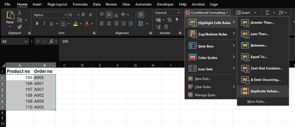
You can do this by following these steps:
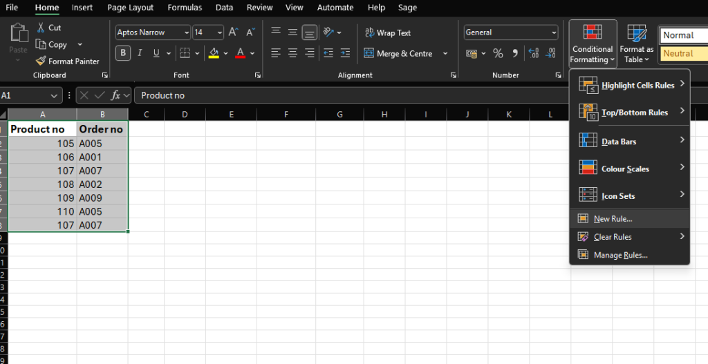
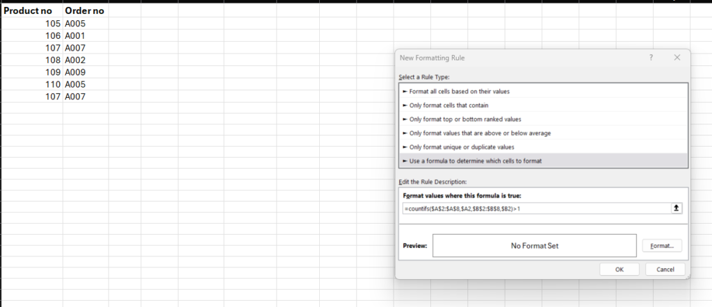
Go to conditional formatting > New Rule.
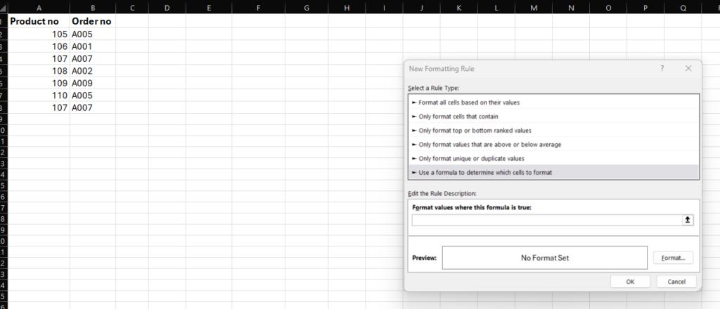
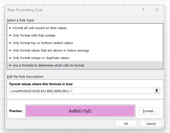
2. Choose ‘Use a formula to determine which cells to format’
3. Enter the formula that you want to use in the box under ‘Format values where this formula is true’.
In this case the formula will be:
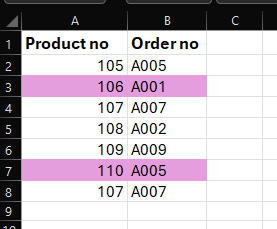
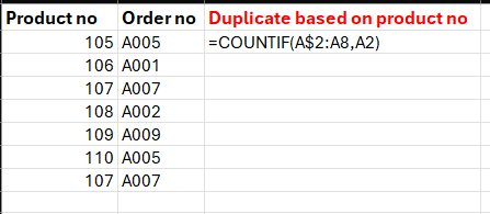
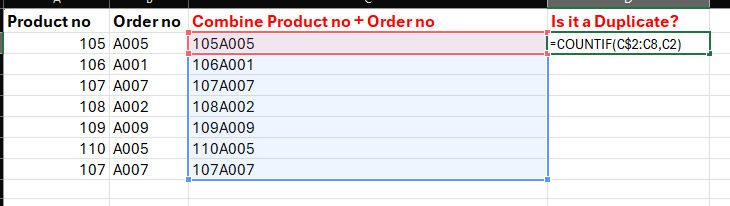
=countifs($A$2:$A$8,$A2,$B$2:$B$8,$B2)>1
Where:
$A$2:$A$8 is the first cell in column A to the last cell in column A where there are values. Or the first cell that you want to compare the second cell to. (Always start from the second cell if the first cell is a heading)
$A2 is the first cell in column A. (Reminder: Always start from the second cell if the first cell is a heading)
$B$2:$B$8 is the first cell in column B to the last cell in column B where there are values. Or the second cell that you want to compare the first cell to.
$B2 is the first cell in column B.
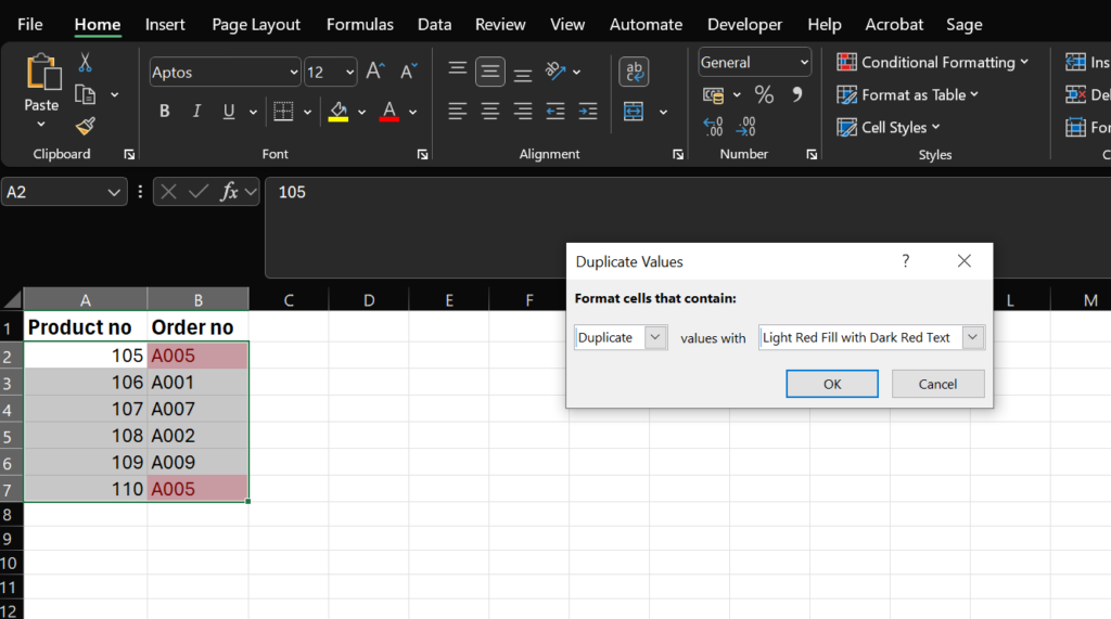
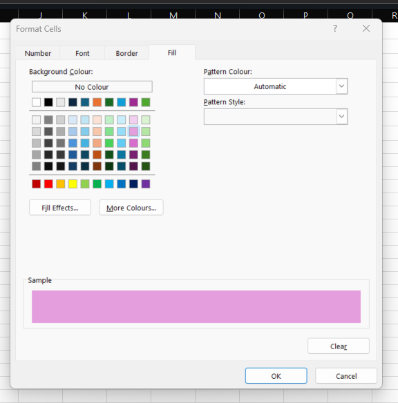
4. Click on ‘format’ and then ‘fill’ to select a color you would like to use to highlight the duplicate rows.
5. Click ‘OK’.
6. The results will then show.
You may also want to see: How to add and subtract a date from today in Excel.
Follow the steps below:
1. In the first cell (C2) of the ‘Duplicate based on product no’ column enter the formula:
=COUNTIF(A$2:A8,A2)
Where:
A$2:A8 is the beginning cell of the column and the last cell of the column.
A2 is the first cell of the column (Reminder: always start from the second cell if the first cell is a heading)
2. Press enter.
3. Copy formula to the rest of the cells in the column by dragging down the tiny block (or double clicking on it) in the bottom right column.
The 1 means it’s not a duplicate and the 2 means that it is a duplicate.
If you need a simple way to check duplicate records without formatting, an Excel formula can help.
To do this, just follow the steps:
Link the 2 columns that you want to use for the comparison with the following formula:
=A2&B2
Where:
A2 is the first cell in the first column and B2 is the first cell in the second column.
2. Add the formula to the rest of the cells in the columns
3. Then compare which cells in column C are duplicates. Enter the following formula is cell D:
= COUNTIF(C$2:C8,C2)
A 1 means that its not a duplicate and 2 means that it is a duplicate.
Let’s see how you can use VLOOKUP to identify duplicates in 2 columns.
Follow the steps below to use VLOOKUP to identify duplicates in 2 columns:
To compare the cells of column A and B enter this formula in column C:
=IFERROR(VLOOKUP(A2,$B$2:$B$8,1,FALSE),””)
You will now be able to see the results in column C.
You may also want to see: How to remove the first or last character in Excel.
Finding duplicate values in two Excel columns doesn’t have to be complicated.
Whether you prefer using Conditional Formatting, formulas like COUNTIF and VLOOKUP, or Excel’s built-in tools, each method helps you quickly clean and organize your data.
By mastering these techniques, you’ll save time, avoid data errors, and improve your overall productivity.
Ready to explore more Excel tips? Check out the related posts linked throughout this guide for even more useful tricks!
You may also want to see How to copy multiple cells in Excel (quick guide).
Important: This post is for informational and educational purposes only. This post should not be taken as therapy advice, financial advice or used as a substitute for such. You should always speak to your own therapist or financial advisor before implementing this information on your own. Thank you!